
Context
In April 2025 I stumbled upon a social media post that showed shadow forecasting for London. They had little icons that indicated whether a place like a bar or restaurant was in the sun or shade and you could move a slider to change the current time and even pick the date.
At the time, they were only covering London and I thought it would be a cool thing to have for Hamburg as well (that's where I live). By now, they cover the entire world, which is not as challenging as it sounds: they are using an API (ShadeMap). However, the API costs $300 per year and I did not want to pay that for my little side project. So I started investigating how to do this from "scratch" (of course, not entirely, since I used tools like QGIS and r.sun.incidout to perform calculations).
While I did not do everything in the most optimal way, I still learned a lot and felt like sharing, which is why I applied to code.talks. Originally, this was intended to be a 45 minute talk, which would have allowed me to go into further detail and actually provide you with a step-by-step tutorial on how to create your own digital surface model and generate shademaps for it. But since we only had 20 minutes I decided to write this little site so you can have all the references you could possibly need to try this out on your own.
In case you have any questions do not hesitate to reach out to me via LinkedIn or mail yanik@schattenpause.de. At the time of writing, it is November the 3rd so my talk is tomorrow and I won't have enough time to update this site to a very polished version and I have no intention of serving you some half-heartedly generated AI-slop so this site will improve in quality over the weekend (Nov 7 & 8).
Data sources
All of the data I used is available for free on Hamburg's Transparenzportal.
City models (CityGML)
- 3D building model LoD1 Buildings as simple blocks with flat roofs
- 3D building model LoD2 Buildings with their actual roof shapes
- 3D building model LoD3 Even more detailed buildings
- Building data on Metaver Alternative download page
Be aware that on the left side of each dataset page you can click on "Newer Version" to get a more recent version of the data.
Terrain & height
- Terrain model (DGM) The ground itself, without buildings or trees
- Digital height model From the LiDAR flyover
- Terrain data on Metaver Alternative download page
Trees
- Street tree register (Straßenbaumkataster) Hamburg's street trees
- Street tree register as JSON Direct download from Hamburg's Geodienste
- Tree data on Metaver The tree data I used
Outside of Hamburg
- Elevation data for Germany (SRTM) OpenDEM
- Building data from OpenStreetMap Overpass Turbo query that exports buildings in a fitting format
Approach
This is roughly how I went from the raw data to actual shadows. It is based on my notes from while I was figuring all of this out, so it is not the most optimal way and some steps are a bit hacky, but it works. Everything happens in QGIS (plus a few GRASS tools that come with it).
All the scripts I mention below are in this GitHub repo, cleaned up a bit and together with a README that explains in which order to run them.
All of Hamburg's data uses the coordinate system EPSG:25832,
so make sure your QGIS project uses it as well.
Digital surface model
To calculate shadows you need a digital surface model (DSM): a raster that contains the height of everything, so terrain and buildings combined.
-
I used the elevation data (
.tif) and the LoD2 building data (CityGML). The elevation data can be imported into QGIS by just drag and dropping it, which results in a raster. -
The elevation data for the whole of Hamburg is split into a lot of
tiles. I wrote a small Python script that finds the tiles that
correspond to a certain region and copies them into a separate
folder. Then use
gdal mergeto merge them into one layer. -
To find the relevant buildings in the CityGML data I simply used
grepwith the postal code of the area I was interested in (you can look up postal codes here):
If you'd rather filter by coordinates, there's a script for that too.grep -rlE 'PostalCodeNumber>(22763)</' path/to/lod2 \ | xargs -I {} cp {} path/to/building-data -
Drag and drop the found
.xmlfiles into QGIS. These need to be converted into polygons: Processing Toolbox → Lines to Polygons. For the polygons you can set a data override for Extrusion under 3D View if you want to look at them in 3D. -
The
measuredHeightof the buildings is relative to the terrain, which means that the terrain would end up with higher values than the buildings and later on you could not differentiate between them. So I added a field with this expression:raster_value('terrain', 1, make_point(x(@geometry), y(@geometry))) + measuredHeight - To combine terrain and buildings, the polygons need to be rasterized via Raster → Conversion → Rasterize. It's important to set the burn-in value to the field with the custom expression from before, so the heights are comparable. For output raster size units I chose georeferenced units and the same resolution as the terrain data (if your data has a 1m raster, which is pretty standard nowadays, enter 1 and 1). Set the output extent to Calculate from Layer and choose the terrain layer.
- For me the Raster Calculator did not work, but the GRASS tool r.series can combine two or more rasters. Select both rasters and choose maximum as aggregate operation: where there is no building you get the terrain, where there is a building its height is higher than the terrain and gets picked. And that's your DSM.
If you want to merge a lot of LoD data at once, QGIS will throw an error because some layers have values in fields that are too long. I wrote a script that refactors the layers to have a max length of 256 for their fields, after that they can be merged inside QGIS.
Trees
Sadly the tree data does not provide the height of the trees, but you
can estimate it using the trunk circumference
(stammumfang). To get the real height, add a field
realHeight with this expression:
raster_value('terrain', 1, make_point(x(@geometry), y(@geometry)))
  + (1.2 + 0.045 * (stammumfang / 3.14159))
When you rasterize the point data directly, the result is just a raster
with 1x1 pixels on the coordinates of each tree. To rasterize them
correctly, first create a field for the radius
(stammdurchmesser / 2), then use Vector → Geoprocessing
Tools → Buffer with a data override on that field for the
distance (15 – 20 segments for the circles work well). After that
rasterize, and the result can be combined with the building and terrain
data just like before.
The tree data covers all of Hamburg, so I used this script to cut it down to the area I was interested in.
Calculating the shadows
For the actual shadows I used the GRASS tool r.sun.incidout with the DSM. Be careful to use the right layer: I tried with the wrong one for a couple of hours and got pretty frustrated after a while. You also need an aspect layer, which you can calculate from the DSM (I think I just used the standard parameters). There is also a GRASS tool, r.slope.aspect, that computes both aspect and slope from the DSM in one go.
The result are four rasters with different information regarding the solar irradiance and stuff, the most important one is the solar incidence angle map. All the no data values are the shadows. So you need to invert the values: every value that is not null becomes 0 and every value that is null becomes 1, so all the shadows have the value 1.
If you then convert the shadow raster to polygons, you can show only
the shadows by going to the layer properties → Source → Query Builder
and using "DN" = 1 as the query.
This script does all of this (plus creating map tiles) inside QGIS in one go.
Smoothing the shadows
r.sun only works with rasters, so the buildings need to be rasterized, which results in pixelated edges and therefore pixelated shadows. There is no real way around this, but you can smoothen the edges a bit by converting the shadow raster into polygons and then applying the Smooth tool.
How long does it take?
It takes approximately 40 seconds to render one image for a local time for a small area like Ottensen. If you calculate in 30 minute steps from 10 am to 8 pm you need 20 images per day, so 40s × 20 = 13 mins 20 secs per day. For a whole month that is 6 h 40 mins.
This does not factor in running things in parallel though. I ran the calculations through a script inside GRASS, and since every area has its own GRASS database you can run several of them at the same time, which was an insane step forward. Another way to speed things up is pre-computing the horizon angles once with the GRASS tool r.horizon and passing them to r.sun (or r.sun.incidout in QGIS, via the horizon parameters). Calculating them takes about 20 minutes for Ottensen, so it's mainly worth it when you calculate a lot of days/times for the same area.
Calling QGIS from the command line was super slow, so I moved the simplifying and tiling back into the Python script. Creating the tiles with QGIS takes about 10 seconds, it might be faster with tippecanoe but at the moment this works best for me.
Bonus: QGIS Python on Mac
After searching way too long I finally found the Python installation
QGIS uses. With its pip you can install custom packages
that you can then use in QGIS:
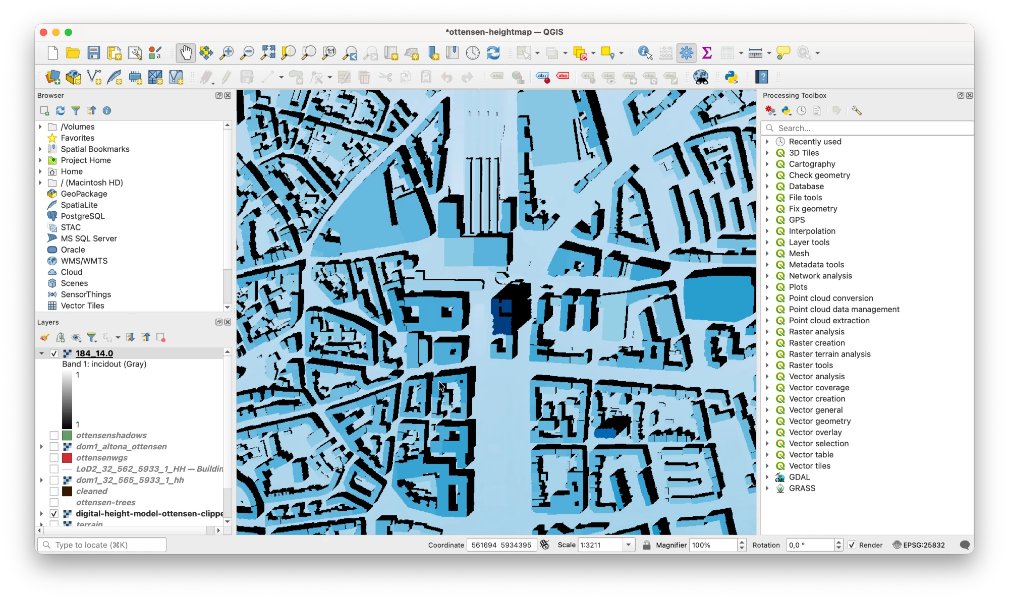
/Applications/QGIS-LTR.app/Contents/MacOS/bin/pip install <package>Screenshot: what the result looks like in QGIS
Other Approaches
There is an approach that I will not be able to cover in my talk which is quite interesting as well. It is similar to what ShadeMap does: the computations of the shadow forecasting happen client-side. If you move around on their site, you will see that after you stop moving it takes a while for the shadows to appear / for the site to become responsive again.
Last year I tried implementing this approach with Claude Code and had no success whatsoever. Now, in anticipation of my talk, I revisited this approach and was able to produce a working demo in a couple of minutes and with a single prompt.
While that is pretty cool I still believe playing around with the stuff and data on your own is way more fun and you actually tend to learn something when looking at this yourself. Yet, to be complete, I wanted to include this approach. This also lowers the entry hurdle to shadow forecasting etc. because you do not have to pay $300 to use the API.
References
- Per Liedman's article liedman.net
- Hamburg's LiDAR flyover Information about how the laser scanning data is collected
- Scripts for this talk Everything I used, cleaned up a bit, on GitHub
- QGIS Free and open source, what I used for pretty much everything
- Hamburg Transparency Law (HmbTG) The reason we have so much cool data
- pyhigh Accessing elevation data in Python
- TessaDEM Elevation API Elevation data via an API
- MapKit Tutorial: Overlay Views Kodeco, for showing shadows on a map in an iOS app
- Advanced MapKit Tutorial: Custom Tiles Kodeco, for serving your own map tiles in an iOS app